ML for SOC-grade network anomaly detection improved between 2022 and 2026 - but not because “Model X beat Model Y” on a benchmark.
The practical leaps are about representations, interaction structure, and operational decisioning (calibration, alert budgets, drift monitoring), under base-rate constraints and adversarial pressure.
Executive summary
Reading note: “What works / fails / hype” are practitioner heuristics under typical SOC constraints (low prevalence, drift, adversarial adaptation). Treat them as default priors, not universal truths - validate in your environment and threat model.
What works (in production reality):
- Treating ML as representation infrastructure (embeddings) that feed multiple downstream detectors and triage workflows.
- Using interaction graphs to detect “coordination anomalies” that per-flow scoring misses.
- Designing an explicit alerting policy (calibration + thresholding + budgets), not shipping raw anomaly scores.
What fails (reliably):
- Closed-world evaluation (random splits, single dataset, no cross-environment tests).
- Global thresholds without drift control (alert storms + gradual irrelevance).
- “Black-box” scoring without investigation hooks (analyst trust collapses).
What’s hype (unless you can prove otherwise):
- “Foundation model generalization” claims without realistic deployment evaluation.
- “Unsupervised = no labels needed” claims without calibration, validation, and a feedback loop.
- Agentic SOC automation without strict sandboxing and auditability.
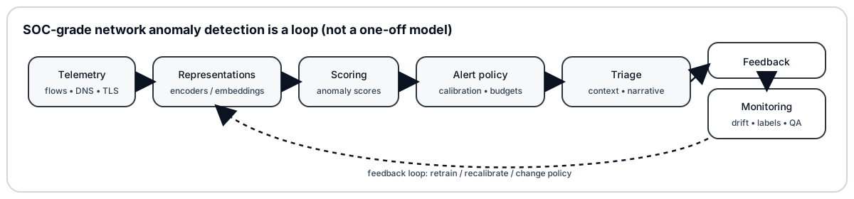
A visual mental model (SOC-grade loop)
1) Why SOC-grade anomaly detection is different
If you take only one idea from this post, make it this:
Security detection is an open-world, adversarial, drifting, low-prevalence problem.
Base-rate reality (why “good ROC” can still be useless)
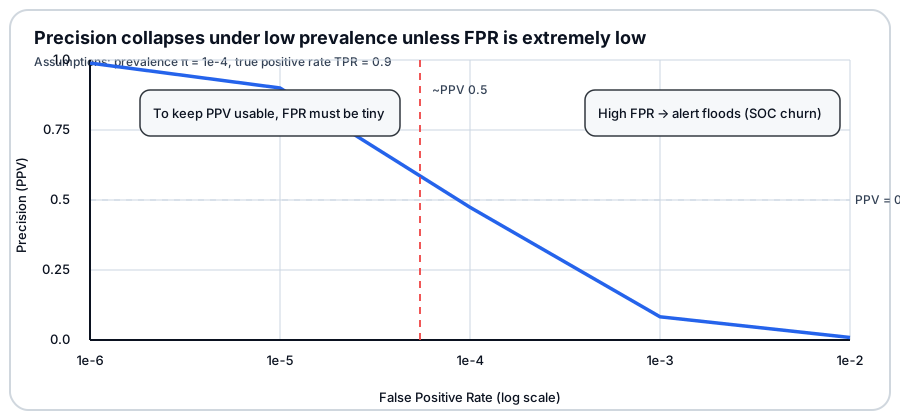
When true incidents are rare, even “great” classifiers drown a SOC in false alarms. The operational metric is precision (PPV) and workload, not a pretty ROC curve.
Let prevalence be $\pi$, true positive rate be $TPR$, and false positive rate be $FPR$:
\[PPV = \frac{TPR \cdot \pi}{TPR \cdot \pi + FPR \cdot (1-\pi)}\]Operational note: $\pi$, $TPR$, and $FPR$ are defined relative to your detector’s scoring unit (flow, session, window, alert-group, etc.). Changing that unit changes prevalence and what “$FPR$” means in practice.
Concrete intuition: when $\pi$ is tiny, you need extremely low $FPR$ to keep $PPV$ usable.
| Example | $\pi$ (prevalence) | $TPR$ | $FPR$ | $PPV$ (precision) |
|---|---|---|---|---|
| “Looks good on ROC” | $10^{-4}$ | 0.90 | $10^{-3}$ | ~8% |
| “SOC-grade-ish” | $10^{-4}$ | 0.90 | $10^{-4}$ | ~47% |
Math note: why “accuracy” doesn’t translate to SOC value
For rare-event detection, you can have high “accuracy” even with a useless detector, because $TN \gg TP$ by default. SOC questions are closer to: - “How many analyst-minutes per true incident found?” - “How many alerts/day does this generate under realistic base rates?”Closed-world evaluation is a default failure mode
Sommer & Paxson’s “Outside the Closed World” remains the best practitioner warning label: your production network is not your curated dataset, and “normal” keeps changing.
The adversary is part of the environment
Attackers observe your detections (or at least their effects), then adapt: they target blind spots in features, thresholds, and labeling workflows. Treat ML detection as a socio-technical system: data + model + people + process.
Key takeaways (problem framing)
- Precision and workload are first-order constraints.
- Drift is inevitable; adversarial adaptation is expected.
- “Unsupervised” still needs governance, calibration, and validation signals.
2) What actually changed in 2022–2026
Three shifts matter most for defenders:
- Representation learning matured for security telemetry (flows, packets, logs, graphs).
- Evaluation culture improved (at least in the best research): more explicit about leakage and realism.
- Decisioning matured: calibration, uncertainty, and alert-rate control became first-class topics.
3) Telemetry is a design choice (especially under encryption)
Encryption moved visibility away from payload into a layered signal stack:
| Layer | Example signals | Typical use | Common failure |
|---|---|---|---|
| Protocol metadata | TLS/QUIC versions, ALPN, SNI, cipher suites | Baselines, grouping | Protocol churn |
| Fingerprints | JA3/JA4 families | Clustering + triage | Not identity; collisions |
| Flow statistics | bytes/packets/duration, burstiness | Cheap baseline | Saturates quickly |
| Sequences | packet sizes/timing, flow sequences | Behavior modeling | Capture-pipeline shortcuts |
| Interaction structure | host↔service/domain graphs | Campaign behavior | Entity resolution errors |
Fingerprints are “interpretable compression”
JA4/JA4+ (newer fingerprint families than JA3) compress protocol configurations into stable-ish identifiers. They’re not magic indicators - but they are high-leverage features for clustering and baselining when combined with time, destination, and endpoint context.
When fingerprinting is not enough: learned representations
ET-BERT is a useful example of the idea that even when payload is hidden, sequence structure and datagram-level patterns can carry discriminative signal.
SOC-grade questions to ask are not “does it classify dataset X?” but:
- Does it generalize across networks and capture pipelines?
- How does it behave under protocol and application evolution?
- Can we monitor it for drift and spurious correlations?
4) Representation learning: from features to encoders
In production, “ML detection” is rarely about the classifier head. It’s about representations:
- what signals exist,
- how you tokenize/aggregate them,
- which invariances you want (site independence, protocol evolution, robustness).
4.1 Self-supervised objectives you actually see in security telemetry
Two common families:
Masked prediction (BERT-style):
\[\mathcal{L}_{MLM} = -\sum_{i \in M}\log p(x_i \mid x_{\setminus M})\]Contrastive learning (InfoNCE-style):
\[\mathcal{L}_{NCE} = -\log \frac{\exp(\text{sim}(z,z^+)/\tau)}{\exp(\text{sim}(z,z^+)/\tau) + \sum_j \exp(\text{sim}(z,z_j^-)/\tau)}\]These losses matter because they let you learn an encoder from abundant unlabeled telemetry, then adapt small heads for:
- alert grouping / deduplication,
- triage enrichment,
- downstream supervised tasks where labels exist.
4.2 Autoencoders: useful baselines, unreliable detectors
Autoencoders are popular because labels are expensive - but reconstruction loss does not guarantee anomalies reconstruct poorly. Treat them as hypothesis generators (outlier surfacing), not autonomous detectors.
Recent work (e.g., Autoencoders for Anomaly Detection are Unreliable) details why reconstruction error is a fragile anomaly signal: models can reconstruct anomalies well, and they can learn shortcuts tied to collection artifacts rather than behavior.
4.3 Transformers for traffic: the interface matters more than the label head
Transformers are valuable when they become reusable traffic encoders. But their “magic” is mostly in the representation interface.
Self-attention (core operation):
\[\text{Attention}(Q,K,V) = \text{softmax}\left(\frac{QK^T}{\sqrt{d_k}}\right)V\]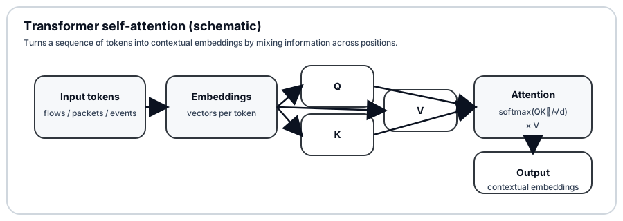
Engineering reality: you must decide what a “token” is (packet, flow, session, event), and which fields to embed (direction, port buckets, timing deltas, JA4, domain categories, etc.).
| Token unit | Example “token” | Best for | Main risk |
|---|---|---|---|
| Flow | 5-tuple + stats + JA4 | scalable baselines | loses within-flow shape |
| Packet burst | sizes + inter-arrival deltas | fine-grained behavior | expensive + pipeline-sensitive |
| Multi-source event | auth + DNS + netflow | SOC narratives | hard normalization |
Deep dive: common tokenization patterns (and trade-offs)
- **Flow-as-token:** scalable, but loses within-flow sequence detail. - **Packet bursts:** captures timing/shape, but can be expensive and capture-pipeline sensitive. - **Event sequences (multi-source):** highest SOC value, but requires normalization + entity resolution.4.4 Foundation models for network security: promising, but evaluation is the bottleneck
Large pretraining efforts (e.g., netFound) suggest a path to reusable encoders across tasks. Two caveats dominate: 1) Data access and privacy: broad pretraining corpora are hard to share. 2) Generalization realism: “works on benchmarks” is not “works across networks.”
Key takeaways (representations)
- Better encoders reduce feature handcrafting, but do not remove base-rate or drift.
- Tokenization/aggregation choices are part of the model (and often the real failure point).
- Strong embeddings without investigation hooks increase MTTR and analyst distrust.
5) Interaction graphs: the most SOC-native representation
Many SOC questions are relational:
- which hosts authenticate to which services,
- which domains co-occur across hosts,
- which processes connect to which destinations.
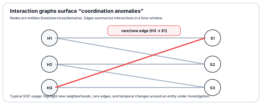
Graph learning matters because it detects coordination anomalies.
Representative directions:
- flow interaction graphs for unknown encrypted threats (e.g., HyperVision),
- inductive GNNs that handle new nodes/edges continuously (e.g., E-GraphSAGE-style patterns),
- temporal contrastive graph learning to learn invariances across windows (e.g., TCG-IDS-style patterns).
5.1 Building a flow interaction graph (practical pattern)
Define nodes as entities (host, user, domain, service) and edges as interactions in a time window.
Pseudocode: build a windowed interaction graph
```text for each time window W: nodes := hosts ∪ domains ∪ services for each flow f in W: u := src_host(f) v := dst_service_or_domain(f) edge(u, v).count += 1 edge(u, v).bytes += bytes(f) edge(u, v).ja4_set.add(ja4(f)) ```5.2 GNN intuition (message passing)
Many practical GNNs can be seen as neighborhood aggregation:
\[h_v^{(k)} = \sigma\Big(W^{(k)} \cdot \text{AGG}\big(\{h_u^{(k-1)} : u \in N(v)\}\big)\Big)\]This aligns with investigation workflows: “what changed in this neighborhood?”
Key takeaways (graphs)
- Graph context turns “anomaly score” into an investigation narrative.
- Graph construction and entity resolution are often the real bottlenecks.
6) Explainability is not a luxury: it’s an operational requirement
A detection is an operational decision: it triggers workflow, containment, and audit trails. An “anomaly score = 0.93” is not a reason.
High-value explainability in SOC tends to be:
- entity-level: which host/user/service drove the score?
- time-localized: what changed in this window?
- contrastive: different from what baseline / nearest neighbors?
- actionable: what evidence should be collected next?
| Explainability artifact | What it answers | “Good enough” output |
|---|---|---|
| Sparse feature deltas | “what drove this?” | top-$k$ features with values |
| Exemplars / neighbors | “similar to what?” | 3–5 comparable historical cases |
| Graph neighborhood diff | “what changed in relationships?” | new/rare edges with timestamps |
| Uncertainty / abstention | “how confident is this?” | calibrated prob. or abstain signal |
Failure modes - explainability
- Score-only alerts: no narrative → no trust.
- Global explanations: irrelevant to the entity/window the analyst is triaging.
- Uncalibrated confidence: “looks certain” under drift, then collapses.
7) Scoring is easy; alerting is hard (calibration + budgets)
You don’t deploy an anomaly score; you deploy an alerting policy.
7.1 Probability calibration: making predicted probabilities reliable
Probability calibration asks whether outcomes assigned probability $p$ occur at about rate $p$ in the relevant population. It applies when the output is intended to be a probability; a ranking or anomaly score need not be one.
Mapping scores to probabilities requires labeled outcomes (or reliable delayed proxies) from a population representative of deployment. Calibration does not by itself stabilize thresholds or reveal drift; threshold selection, alert-rate control, and drift monitoring remain separate operational controls.
Common probability-calibration tools include:
- Platt scaling (logistic calibration)
- isotonic regression
When you have labels (or reliable proxies), the Brier score is a useful proper scoring rule for probabilistic predictions:
\[\text{Brier} = \frac{1}{n}\sum_{i=1}^n (p_i - y_i)^2\]It reflects both calibration and resolution, so assess calibration itself with reliability diagrams or an explicit calibration-error analysis rather than treating Brier as a pure calibration metric.
7.2 Conformal prediction: coverage, not probability calibration
Conformal prediction wraps a model to produce prediction sets or intervals. Under exchangeability of the calibration examples and a new example, a standard conformal procedure targets marginal coverage:
\[\Pr\!\left\{Y_{\mathrm{new}} \in C_\alpha(X_{\mathrm{new}})\right\} \ge 1-\alpha\]Empty or multi-label sets can support an abstention policy, but this guarantee does not turn a classifier’s scores into calibrated class probabilities. In drifting or time-dependent telemetry, exchangeability is especially fragile; coverage must be monitored and the conformal method adapted to the stream.
7.3 EVT thresholding (tail modeling for alert-rate control)
EVT methods like SPOT model the tail of a score stream to place thresholds with explicit risk parameters.
If exceedances over a high threshold $u$ follow a Generalized Pareto Distribution (GPD), tail probabilities can be controlled via fitted parameters $(\xi, \beta)$.
Operationally, EVT/SPOT is an alert-rate / tail exceedance control tool under stationarity assumptions; it does not, by itself, guarantee usable $PPV$. In practice you still need backtesting, refitting, and seasonality/non-stationarity handling.
7.4 Online FDR control (treat alerts as multiple testing)
Online false discovery rate control reframes “alert or not” as sequential hypothesis testing - useful when you want explicit control of “fraction of alerts that are noise” over time.
This relies on a defensible score→p-value mapping and assumptions about dependence; treat it as a governance layer, not a quality guarantee.
| Decisioning method | What it controls | Why it helps SOC | When it breaks |
|---|---|---|---|
| EVT/SPOT-style | tail risk / alert rate | alert budget stability | non-stationary tails |
| Conformal | marginal coverage of sets / intervals | explicit uncertainty sets and abstention | exchangeability fails; sets can be uninformative |
| Online FDR | false discoveries over time | workload governance | weak p-value modeling |
Key takeaways (decisioning)
- Single global thresholds fail under drift and changing prevalence.
- Probability calibration and conformal coverage are different deliverables with different assumptions.
- Alerting should be governable with explicit assumptions and monitoring.
8) Drift: accuracy decay and meaning decay
Drift is not an edge case - it’s the default.
Two kinds of drift matter operationally:
- accuracy drift: the model’s predictive power degrades
- meaning drift: the “story” behind alerts changes (new SaaS rollout, new user behavior)
Guardrails often look like: drift detection + alert-volume monitors + precision proxies (e.g., analyst-confirmed rate, suppression rates).
Deep dive: Page-Hinkley drift test (one common pattern)
One common one-sided form for detecting sustained increases updates the mean and cumulative deviation recursively. Initialize $\hat{\mu}_0=S_0=M_0=0$; for $t\ge1$: $$ \begin{aligned} \hat{\mu}_t &= \hat{\mu}_{t-1} + \frac{x_t-\hat{\mu}_{t-1}}{t},\\ S_t &= S_{t-1} + \left(x_t-\hat{\mu}_t-\delta\right),\\ M_t &= \min(M_{t-1},S_t). \end{aligned} $$ Define $PH_t=S_t-M_t$ and signal a change when $PH_t>\lambda$. The current mean is used once in the time-$t$ increment; it is not substituted retroactively into every earlier summand. Here $\delta$ is the tolerated change and $\lambda$ is the alarm threshold. For sustained decreases, initialize $S^-_0=M^-_0=0$ and use the explicit mirrored statistic: $$ S^-_t = S^-_{t-1} + \left(x_t-\hat{\mu}_t+\delta\right), \qquad M^-_t = \max(M^-_{t-1},S^-_t), \qquad \text{signal if } M^-_t-S^-_t>\lambda. $$ Equivalently, apply the increase detector above to $-x_t$.9) Adversarial pressure: threat model the detector and the pipeline
You don’t need Hollywood “AI attacks” to be in adversarial ML territory - pipeline attacks and workflow manipulation are more realistic.
| Risk surface | Defender question | Typical control (high-level) |
|---|---|---|
| Label workflow | “Can an attacker influence labels?” | separation of duties, review gates |
| Data pipeline | “Can collection be spoofed?” | integrity checks, anomaly on telemetry quality |
| Model outputs | “Can scores be probed/extracted?” | rate limits, access control, output hardening |
| Drift/adaptation | “Can adaptation lock in poison?” | retrain gates, rollback plans, canaries |
Use shared language for reviews (NIST AML taxonomy; MITRE ATLAS) and treat ML artifacts like any other production dependency.
10) Governance and pipeline security
If you deploy ML in detection, you’re deploying a socio-technical system: data + model + people + process.
A practical governance lens is NIST’s AI RMF (GOVERN, MAP, MEASURE, MANAGE). In SOC terms:
- MAP: define threats, assets, blast radius, and operational constraints (alert budget, SLAs).
- MEASURE: monitor performance, drift, calibration, and label health.
- MANAGE: retrain gates, rollbacks, and incident response for the ML pipeline itself.
Security controls (conceptual checklist):
- data lineage & integrity (collection → storage → features),
- separation of duties (who can change features/thresholds/models),
- immutable evaluation artifacts (reproducible experiments),
- drift monitoring and alert-volume monitors,
- audit logs for any automation (especially LLM/agent tools).
Failure modes - governance
- No rollback: the model becomes an unpatchable dependency.
- Unowned drift: nobody is accountable for “when to retrain / when to freeze.”
- Shadow automation: copilots without auditability become compliance risk.
11) Evaluation without self-deception
Minimum bar for SOC-grade evaluation:
- temporal splits (no future leakage)
- cross-environment tests (different sites/segments/capture pipelines)
- operational units (alerts/day, analyst-minutes/incident), not just AUC
- explicit reporting under realistic base rates (precision is prevalence-dependent)
Deep dive: why PR beats ROC under extreme imbalance
Precision and recall: $$ \text{Precision} = \frac{TP}{TP+FP}, \quad \text{Recall} = \frac{TP}{TP+FN} $$ ROC can look great even when $FP$ volume makes the detector unusable. PR surfaces that operational reality.Operational math: from FPR to alerts/day
If your system evaluates $N$ mostly-benign events/day, expected false alerts/day is roughly: Here, “events” means whatever items you score and could alert on (flows, sessions, windows, host-days, alert-groups, …). $$ FP/day \approx FPR \cdot N $$ With $N=50{,}000{,}000$ events/day: - $FPR=10^{-4}$ → ~5,000 false alerts/day - $FPR=10^{-5}$ → ~500 false alerts/day That’s why “small” $FPR$ values still matter massively at scale.12) Frontiers: what looks promising (and what’s just hype)
12.1 Multimodal detection (the missing integration layer)
In security, “multimodal” means network + endpoint + identity + graph context. The best systems are hybrid:
- ML for representation + scoring
- rules/signatures for hard constraints and known-bad
- graphs for context
- LLMs for summarization and workflow support (not the primary detector)
12.2 LLMs and agents in SOC
LLMs tend to add the most value in the human layer:
- summarization and case notes
- normalizing vendor vocabularies
- retrieval-augmented investigation
Agentic automation should be treated as privileged code: sandbox tools, minimize permissions, and audit everything.
13) A practical reference architecture (SOC-grade)
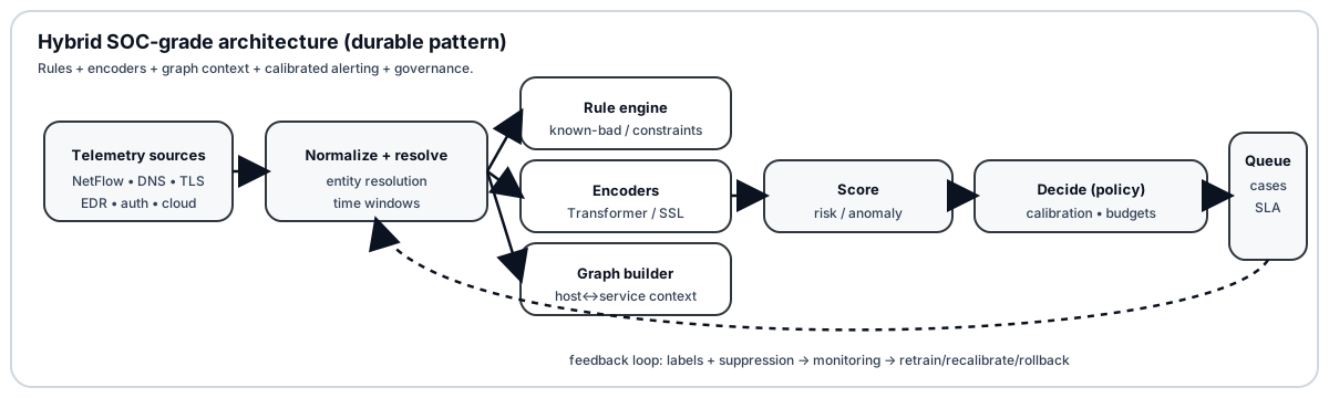
A durable pattern:
- Build stable telemetry + entity resolution.
- Train or adopt reusable encoders (flow/sequence/graph).
- Make alerting controllable (calibration + thresholds + budgets).
- Add investigation hooks (context, neighbors, prototypes).
- Run drift monitoring + retraining gates with rollback.
14) A critical perspective (what we still get wrong)
Three persistent traps
1) “Unknown attacks” is not one category. Unknown could mean:
- novel malware family on known infrastructure,
- known technique on a new protocol stack,
- benign-but-rare change in your environment,
- a slow campaign hiding in normal variability.
2) Reproducibility and operationalization are bottlenecks. Production needs:
- stable pipelines and feature availability,
- monitoring and retraining mechanics,
- governance, auditability, and change management,
- integration with case management and response tooling.
3) Accuracy is not the metric you think it is. A practical north star is:
- analyst-minutes per true incident found,
- with explicit alert budgets and drift tracking.
Glossary
- Alert budget: a target cap on alerts per unit time (and/or per analyst), used to keep detection governable under drift.
- Probability calibration: mapping scores intended as probabilities so predicted probabilities agree with observed frequencies, usually requiring labels or reliable proxies.
- Conformal prediction: constructing prediction sets or intervals with a coverage guarantee under assumptions such as exchangeability; it does not itself calibrate class probabilities.
- Encoder / embeddings: a model that maps raw telemetry into vectors used by multiple downstream tasks (clustering, retrieval, classification).
- Entity resolution: matching IDs across telemetry so “host/user/service/domain” refer to consistent entities.
- EVT / SPOT: thresholding via tail modeling to control exceedance/alert rates under stationarity assumptions.
- FDR (false discovery rate): expected fraction of false discoveries among discoveries; “online FDR” controls this sequentially under assumptions.
- FPR: probability of flagging benign items as suspicious (depends on the scoring unit and decision policy).
- Interaction graph: a graph where nodes are entities and edges are observed interactions within a time window.
- JA3/JA4: JA3 is a TLS ClientHello fingerprint; JA4/JA4+ is the successor family of fingerprints covering TLS, QUIC, and other protocols. Both are used as features for clustering/baselining (not identities).
- PPV / precision: probability an alert is truly positive given it fired (depends on base rate).
- Scoring unit: what you assign a score to (flow, session, window, host-day, alert-group, …); it defines prevalence and alert volume.
- Tokenization (in this post): how telemetry is turned into model inputs (“tokens”), e.g., flows, packet bursts, or multi-source events.
- TPR / recall: probability of catching a true positive when it occurs, relative to a chosen definition of “positive.”
References
Reality checks & evaluation
- Stefan Axelsson - The Base-Rate Fallacy and its Implications for the Difficulty of Intrusion Detection (CCS 1999)
- Stefan Axelsson - The Base-Rate Fallacy and the Difficulty of Intrusion Detection (ACM TISSEC 2000)
- Robin Sommer, Vern Paxson - Outside the Closed World (IEEE S&P 2010)
- Daniel Arp et al. - Dos and Don’ts of Machine Learning in Computer Security (USENIX Security 2022)
- Takaya Saito, Marc Rehmsmeier - The Precision–Recall Plot Is More Informative than the ROC Plot… (PLOS ONE 2015)
Representations (Transformers, graphs, robustness)
- Xinjie Lin et al. - ET-BERT (WWW 2022)
- Satyandra Guthula et al. - netFound (arXiv 2310.17025)
- L. D. Manocchio et al. - FlowTransformer (Expert Systems with Applications, 2024)
- C. Fu et al. - HyperVision (NDSS 2023)
- Y. Qing et al. - RAPIER (NDSS 2024)
- R. Bouman, T. Heskes - Autoencoders for Anomaly Detection are Unreliable (arXiv 2501.13864, 2025)
- W. W. Lo et al. - E-GraphSAGE: A GNN-based IDS for IoT (arXiv 2103.16329)
- C. Wu et al. - TCG-IDS: Robust Network Intrusion Detection via Temporal Contrastive Graph Learning (IEEE TIFS, 2025)
- Ł. Korycki, B. Krawczyk - Adversarial Concept Drift Detection under Poisoning Attacks… (2022)
Thresholding, drift, and statistical control
- E. S. Page - Continuous Inspection Schemes (Biometrika, 1954)
- D. V. Hinkley - Inference about the Change-Point from Cumulative Sum Tests (Biometrika, 1971)
- Anastasios N. Angelopoulos, Stephen Bates - Conformal Prediction: A Gentle Introduction (Foundations and Trends in Machine Learning, 2023)
- Alban Siffer et al. - Anomaly Detection in Streams with Extreme Value Theory (SPOT) (KDD 2017)
- E. Krönert et al. - FDR Control for Online Anomaly Detection (arXiv 2312.01969)
- Shuo Yang et al. - ReCDA (KDD 2024)
Adversarial ML, governance, and GenAI risks
- NIST - AI RMF 1.0 (NIST AI 100-1)
- NIST - Adversarial Machine Learning: A Taxonomy and Terminology… (NIST AI 100-2e2025)
- MITRE - ATLAS (Adversarial Threat Landscape for AI Systems)
- OWASP - Top 10 for Large Language Model Applications (2025)
Encrypted traffic signals (fingerprints)
- FoxIO - JA4+ Network Fingerprinting (specs & code)
- Cloudflare - JA4 fingerprints and inter-request signals
- Suricata - JA4 keywords documentation